Interpolate

Introduction

Interpolate can generate predicted values for a specified area based on the input sampled values.

1. Set the input data

• Input Data: Spatial data only.

2. Select the interpolation field

• Interpolation Field: Its value will be calculated for the spatial extent of the input data.

3. Set the output cell size

• Output Cell Size: The side length of a square cell in the output data. A value will be calculated for each cell.

4. Set the output data

• Output Data Name: If no name is set, the default is "toolName_time".

5. Submit

After completing the above settings, click Submit to start the tool.
When it finishes successfully, a message will be shown at the top of the page. You can click the Open Data button to start accessing the data or go to the Data page to view it.

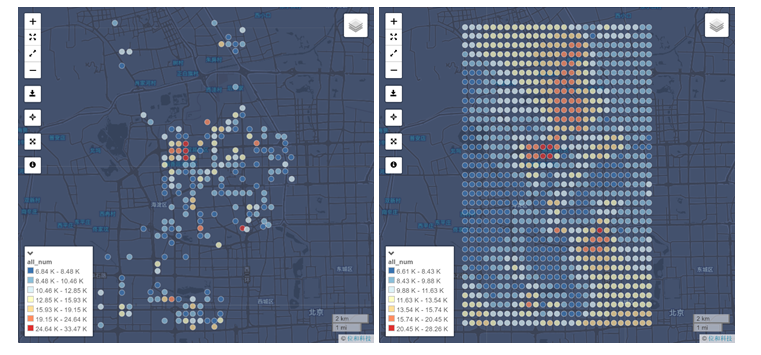
The figures below shows the difference between the original population distribution map and the population distribution map processed by Interpolate function. The second map can clearly demonstrate the continuous population distribution over an entire area.

Kriging Interpolation and Advanced Settings

Commonly, a spatial unit is similar to other adjacent spatial units within a continuous space. As the distance between units decreases, the corresponding difference will also diminish. The difference calculation consists of the spatial tendency, the spatial autocorrelation, and the stochastic error term. Spatial tendency is a structure factor within a big space, for example, the house price is decreasing from urban areas to suburban areas. Spatial autocorrelation is a structure factor within a small space, for example, the house price is relatively higher if the house is close to the subway station. Based on these spatial factors, Kriging Interpolation can estimate the attribute value of an unknown point. The approximate value is a weighted average value of the adjacent known points.

‌If the distance between two points increases, the corresponding difference will also rise and it can be represented by the semi-variance value. Semi-variance value is the average difference between two points with the same distance and semi-variance function is the function calculating the change of the semi-variance. As the distance increases, the semi-variance will also rise; subsequently, the Kriging Interpolation will build the relationship between the attribute values of each point to estimate the information of the unknown points.

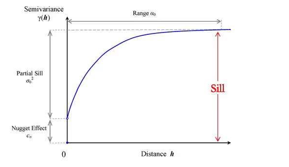
The figure above is the diagram of semi-variance function, in which, there are three important parameters (Nugget, Sill, and Range)

Nugget: the difference between the spatial points in the initial stage of the semi-variance function. Conceptually, the semi-variance should be zero when the distance is also zero; however, the spatial variance caused Nugget effect to have an initial difference

Sill: the maximum semi-variance in the diagram and Partial Sill value is Sill value minus the block gold value.

Range: the maximum distance between two related points, in other words, the maximum distance when the semi-variance function reaches Sill value.

You can use advanced settings to specify the parameters above.